Evaluating the performance of COVID-19 rapid tests
Note that in the early days of the 2020 pandemic there was a lot of uncertainty regarding the effectiveness of the rapid tests. This was an attempt at quantifying the performance of the different tests present in the market.
In this project, I developed a framework to quantify the uncertainty surrounding the performance of several Sars-CoV-2 rapid serological tests. This allows to:
- given the results of a population study, to correct the results for false positives and false negatives, in a test-specific manner, in order to obtain accurate estimates of the real prevalence of seropositives, together with a measure of its uncertainty.
- to make informed decisions about the choice of test to use, when planning studies
I used to the data reported to the US Food and Drug Administration (FDA) by the manufacturers to quantify the sensitivity and specificty of each test, together with the uncertainty associated with it. From here, we write the observed frequency of sero-positive results in a study as a function of the actual prevalence, the rate of false positives, and the rate of false negatives:
\[ p_{\textrm{obs} } = p_{prev}\cdot (1-p_\textrm{fnr}) + (1- p_\textrm{prev} ) \cdot p_\textrm{fpr} \]
where:
- \(p_{\textrm{obs} }\) is the observed frequency of positives
- \(p_{prev}\) is the real prevalence
- \(p_\textrm{fnr}\) is the rate of false negatives
- \(p_\textrm{fpr}\) is the rate of false positives
So, essentially, this formula is saying that the observed frequency of positives (\(p_\textrm{obs}\)) is the real positives times the true positive rate (discounting false negatives) plus the number of negatives times the false positive rate.
We then include this formula in a Bayesian framework, that assigns this probability of observing positives to a Binomial distribution, as well as the numbers of the diagnotics test (numbers and totals of false positives and false negatives). This model jointly estimates false positive and negative rates, together with the real prevalence and the joint uncertainty. We wrap this as a pymc model, that allows us to sample the posterior distribution using NUTS, the state of the art Hamiltonean Monte-Carlo sampler.
Comparing test-specfic distortions
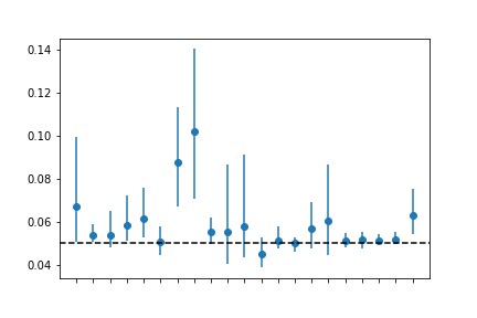
One thing we can do to illustrate the differences between tests, is to see what the real prevalence would be for the same number of observed positives (figure Figure 1 ).

Alternatively, one can simulate data, assuming one real prevalence, and running it through the several tests to see what the reported rate of positives would be for each test.